Olena Orlova (2022). Idiosyncratic preferences in games on networks. Games and Economic Behavior 131: 29–50.
How do our social connections—or, more generally, the structure of our social networks—influence how we make decisions? The dominant approach in the theory of networks takes this to be a question exclusively about network effects. On this view, what we (optimally) do is a function of an underlying network structure: my preferences over coffee and tea, say, depend on the choice of beverage that my friends, or acquaintances, make as well as on how much, and in what way, I care about these social connections. If I like my friends, for example, then the more they drink coffee, the more likely I may be to (optimally) drink coffee as well—our actions, in this case, would be strategic complements. Alternatively, if I dislike my friends, the more they drink coffee, the more likely I may be to go for tea—a situation of strategic substitutes.
Understanding the network effects of individual decision making is immensely important but focusing only on these effects is a different matter. Such an approach, as Olena Orlova points out, ultimately assumes that the only source of heterogeneity between agents—relevant to decision making, that is—is that of their network position. Such an approach thus abstracts away from any non-network-related differences in our preferences. My choice of beverage may be a function of my friends’ drinking habits, but it may also depend, in part, on my (exogenously given) preferences over coffee and tea. (One may be tempted to phrase this distinction as one of personal vs structural heterogeneity, but this is too crude—after all, how a network structure affects an agent’s decision making may vary across agents and may thus carry some personal heterogeneity.) Surprisingly, especially given the history of economic thought, attention to how the unique preferences of agents affect what they do in social networks has been sparse (see the discussion on 31 for some related work; most of the preference-related work has been on ‘strategic network formation’, which deals with how preferences affect the formation, and thus structure, of a network). Analysing the interaction between these two sources of agential heterogeneity is the main contribution of Orlova’s paper. It is important to stress that this contribution does not consist in extending or generalising the standard framework. As Orlova points out (43–44), the equilibria in the standard framework are neither a subset nor a superset of those in the more complex framework. In this sense, introducing preference heterogeneity in the standard case leads to a substantively distinct framework that needs to be analysed on its own terms (though some ‘degenerate’ results, pointed out below, do carry over)—this is where Orlova’s contribution lies.
The motivation
To get a sense of this contribution and why it is important, consider the following example. There are five agents, \(A\), \(B\), \(C\), \(D\), and \(E\), in a social network that can be illustrated as follows (for now, focus on the left panel; the example is adapted from the one on 38):
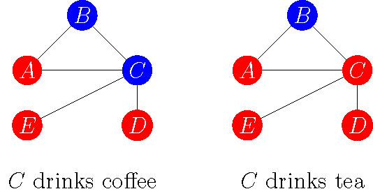
Suppose that a link between two agents refers to the existence of a friendship (as the network is undirected, friendship is reciprocal: if \(A\) is friends with \(B\), \(B\) is also friends with \(A\)). For instance, in this network, \(A\), \(B\), and \(C\) are a close-knit group where every agent is friends with every other agent, while \(C\), clearly the most popular agent, is friends with everyone. Suppose, further, that each agent may do either of two things: (1) drink coffee (indicated in blue), or (2) drink tea (indicated in red). Then consider the situation depicted in the left panel above, where \(B\) and \(C\) drink coffee and \(A\), \(D\), and \(E\) drink tea.
To be able to say something about individual utility in this situation, we need to know how utility is affected by one’s friendship network. Suppose that for each immediate friend who drinks the same (different) beverage, the respective agent receives a utility of \(1/3\) (\(2/3\)). Thus, in the left network above where agent \(C\) drinks coffee, \(C\)’s utility is \(2/3+1/3+2/3+2/3=7/3\). Conversely, in the right network above where \(C\) drinks tea, \(C\)’s utility is \(1/3+2/3+1/3+1/3=5/3\). Clearly, in the situation where \(A\), \(D\), and \(E\) drink tea while only \(B\) drinks coffee, \(C\) is better off drinking coffee. Notice that, in this example, \(C\) cares more about ‘mis-matching’ her action with those of her friends (‘mis-matching’ has a payoff of \(2/3\), which is bigger than the ‘matching’ payoff of \(1/3\)). We are thus in a game of strategic substitutes. That is, \(C\) is better off drinking coffee in such a situation because most of her friends are drinking tea and \(C\) prefers drinking something different. (\(C\) is friends with everyone but is a bit of a contrarian.)
One drawback of the utility function above is that it is entirely dependent on what Orlova calls ‘interactional utility’: the part of one’s utility function that captures network effects. It ignores however, in Orlova’s words, one’s ‘idiosyncratic utility’: the part of one’s utility function that captures one’s idiosyncratic preferences (here, over coffee and tea). Orlova’s contribution is to combine these two components in an overall utility function that captures both network and idiosyncratic effects.
To appreciate why combining these effects might be important, let’s now distinguish between the actions agents may take (drink coffee or tea) and their exogenously given, idiosyncratic preferences over these actions (prefer coffee or tea). Consider the following variation on the situation above:
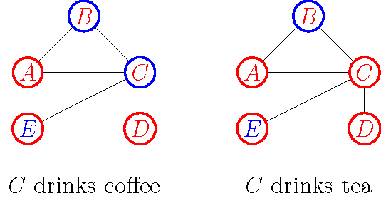
Here, the colour of the outline of a node indicates the actions in the respective situation: for example, on the left, it is still the case that \(A\), \(D\), and \(E\) drink tea while \(B\) and \(C\) drink coffee. The colour of the letter in a node now indicates that agent’s idiosyncratic preference: for example, on the left, \(E\) prefers coffee (to tea) while \(A\), \(B\), \(C\), and \(D\) prefer tea (to coffee). Suppose that ‘mis-matching’ still carries a (relative) benefit of \(2/3\) while ‘matching’ yields a (relative) benefit of \(1/3\). But now further suppose that, in any situation where an agent performs the action she prefers, she gets a benefit of \(1/4\) for each of her friends; otherwise, when she does not perform her preferred action, she gets a benefit of zero. When \(C\) drinks coffee (left panel), \(C\)’s utility is \(2/3+1/3+2/3+2/3=7/3\). When \(C\) drinks her preferred beverage, tea (right panel), her utility is \(1/3+2/3+1/3+1/3+4/4=8/3\). And so \(C\) is better off drinking tea.
The important thing to notice here is that interactional and idiosyncratic utility may pull in different directions. \(C\) may be a contrarian but if she cared enough about her idiosyncratic tastes, then she may be better off going for what her friends do if that were what she cares about. Alternatively, \(C\) may not have strong beverage preferences—if going for her preferred drink were worth just, say, \(1/12\) per friend, \(C\) would be better off being contrarian and drinking coffee.
Preferences over and choices of beverage are innocent enough, but other contexts reveal how important understanding these interactional effects is. Orlova gives the example of school choice (30): in the illustration above, the agents could be parents who are friends or part of a neighbourhood; their actions could be the school (one of two) they choose for their children and their idiosyncratic preferences could be their preferences over these schools. School choice, especially among tight friendship or neighbourhood networks, has wider segregation effects—understanding when parents in a close network coordinate on the same school is essential for understanding how segregation may arise and be maintained. The two, among others, classes of games that Orlova focuses on—coordination games, where agents adopt the same action, and anti-coordination games, where agents choose different actions—are immensely relevant here.
In passing (30n6), Orlova mentions that idiosyncratic preferences may also be interpreted as identities. In fact, I think we can go further and interpret the whole model as a model of identity choice. The groups, broadly construed, that we decide to become members of depend both on idiosyncratic values we hold and on group effects (say, status or group benefits). Understanding the interaction between these two sources of identification is then helpful for understanding the conditions under which we end up with ‘narrow’ or ‘broad’ (or ‘multiple’) identities. (See Partha Dasgupta and Sanjeev Goyal’s model of narrow identities and this symposium on the paper.) These cases would correspond to coordination and anti-coordination games and so the bridge between Orlova’s model and the economic literature on identity choice is an easy one to build.
In order to summarise the main insights of Orlova’s paper, and discuss some of its wider implications, we need a couple of preliminaries.
Preliminaries
A network, like the one(s) above, is a pair \((N,G)\), where \(N=\{1,\dots,n\}\) is a set of nodes (or agents) and \(G\) is an adjacency matrix indicating the (undirected) links between the agents. Thus, \(G_{ij} \in \{0,1\}\) for all agents \(i,j \in N\), where \(G_{ij}=0\) means that there is no link between \(i\) and \(j\) (above, that they are not friends) and \(G_{ij}=1\) means that there is (above, that they are friends). For example, for the networks we’ve seen so far, we have \(N = \{A,B,C,D,E\}\) and \(G_{Ci} = 1\) for \(i \in \{A,B,D,E\}\). Collect in set \(N_{i}(G) = \{j \in N \ | \ G_{ij}=1\}\) all agents to which \(i\) is connected (above, is friends with) and let \(d_{i}\) denote the cardinality of (the number of members in) this set (above, the number of \(i\)’s friends). For instance, \(N_{C}(G) = \{A,B,D,E\}\) and \(d_{C}=4\). Each agent has one of two actions, denoted by \(x_{i} \in \{0,1\}\), and each agent has a preference for one of the two actions, denoted by \(\theta_{i} \in \{0,1\}\). The vectors \(\mathbf{x}\) and \(\mathbf{\theta}\) denote arbitrary action and preference profiles, respectively. For simplicity, the \(d_{i}\)-tuple \(\mathbf{x}_{N_{i}(G)}\) denotes the actions of \(i\)’s friends under \(\mathbf{x}\).
We can now define the interactional utility function Orlova works with. For any \(i \in N\), it has the following form (32):
\(u_{i}(\theta_{i}, x_{i}, \mathbf{x}_{N_{i}(G)}) = \sum_{j \in N_{i}(G)} \left( \delta \cdot \mathbb{1}_{x_{i}=x_{j}} + (1-\delta) \cdot (1 - \mathbb{1}_{x_{i}=x_{j}}) + \lambda \cdot \mathbb{1}_{x_{i}=\theta_{i}} \right)\)
Where \(\delta \in [0,1]\) is the ‘matching’ benefit (and \(1-\delta\) is the ‘mis-matching’ benefit) and \(\lambda \in [0,\infty)\) is the benefit an agent obtains from following their idiosyncratic preference. Here, \(\mathbb{1}_{x_{i}=x_{j}}\) is an indicator function that is equal to one when \(j\)’s action matches \(i\)’s, and zero otherwise. (And so \(1 - \mathbb{1}_{x_{i}=x_{j}}\) is equal to one when \(j\)’s action mis-matches \(i\)’s, and zero otherwise.) Similarly, \(\mathbb{1}_{x_{i}=\theta_{i}}\) is equal to one when \(i\)’s action matches her preference, and zero otherwise. When \(\lambda = 0\), we are in the canonical case where only network effects influence individual utility, while when \(\lambda\neq 0\), we are in the case of interactional utility where idiosyncratic preferences also play a role. Finally, when \(\delta > 1/2\), matching has a bigger (marginal) benefit than mismatching and so we are in the case of strategic complements; conversely, \(\delta < 1/2\) is the case of strategic substitutes. (Recall that, in the example above, we had \(\delta=1/3\) and \(\lambda=1/4\).)
Given this set-up, values for \(\delta\) and \(\lambda\) define distinct games, which is why Orlova refers to a game as \((\delta,\lambda\)). Furthermore, by introducing a tie-breaking rule, we may rule out mixed Nash equilibria, allowing us to focus on pure equilibria. Orlova does just that by requiring that whenever an agent is indifferent between two strategies, she go with her idiosyncratic preference. She calls this refined Nash equilibrium concept a selfish Nash equilibrium (32).
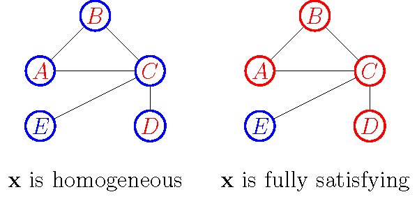
There are (at least) two types of situations that are particularly intriguing in this setting. First, equilibria where all agents adopt the same action—in Orlova’s words, these are homogeneous equilibria (otherwise, they are called heterogeneous). Second, equilibria where all agents adopt the action that coincides with their idiosyncratic preference—in Orlova’s words, these are fully satisfying equilibria (otherwise, they are called frustrating). For instance, in
Coordination games
Consider first the case of coordination games where \(1/2 < \delta \leq 1\) and \(0 < \lambda < 2\delta -1\) (33). That is, in such games, (1) the matching benefit \(\delta\) is stronger than the mismatching benefit \(1-\delta\) and (2) the stronger the matching benefit \(\delta\) is (the closer it is to one), the wider the admissible range of idiosyncratic benefits \(\lambda\) is (conversely, the weaker \(\delta\) is, the smaller the admissible range of \(\lambda\) is). Notice, in particular, that \(2\delta - 1\) is the (least) upper bound of the idiosyncratic benefit—in other words, for a game to be a coordination game, on this definition, the strength of the idiosyncratic benefit should be bounded from above by the strength of the matching benefit. Consider the five-agent network illustrated so far, which we may describe by its degree distribution, that is, the distribution of connections (above, friends) that each player has. In our example, we have agents with a degree of \(1\) (agents \(D\) and \(E\)), \(2\) (agents \(A\) and \(B\)), and \(4\) (agent \(C\)). Notice that an agent’s utility here depends on how many of her neighbours perform the same action as she does and whether that action is her preferred action. Call an agent’s neighbour who performs her preferred action her companion (33). For example, in the left panel of
Consider, first, the agents of degree \(1\) (agents \(D\) and \(E\)). For arbitrary \(\delta\) and \(\lambda\) that satisfy the coordination-game conditions, the minimum number of companions such agents need for their preferred action to be optimal is given by:
(1) \(l_{\delta,\lambda}(1) = \lambda + 2 \delta - 1\) when \((2\delta -1)\frac{1-2(2\delta-1)}{1+2(2\delta-1)} \leq \lambda < 2\delta-1\) (that is, when \(\lambda\) is ‘sufficiently close’ to its upper bound);
(2) \(l_{\delta,\lambda}(1) = \lambda + 2 \delta\) when \(0 < \lambda < (2\delta -1)\frac{1-2(2\delta-1)}{1+2(2\delta-1)}\) (that is, when \(\lambda\) is ‘sufficiently smaller’ than its upper bound).
For agents of degree \(2\) (agents \(A\) and \(B\)), we have:
(1) \(l_{\delta,\lambda}(2) = \lambda\) when \((2\delta -1)\frac{1}{2\delta} \leq \lambda < 2\delta-1\) (that is, when \(\lambda\) is ‘sufficiently close’ to its upper bound);
(2) \(l_{\delta,\lambda}(2) = \lambda + 1\) when \(0 < \lambda < (2\delta -1)\frac{1}{2\delta}\) (that is, when \(\lambda\) is ‘sufficiently smaller’ than its upper bound).
And, finally, for agent (C) of degree (4), we have:
(1) \(l_{\delta,\lambda}(4) = \lambda - \frac{2\delta - 1}{2}\) when \((2\delta -1)\frac{2 + \frac{2\delta-1}{2}}{2 + 2\delta - 1} \leq \lambda < 2\delta-1\) (that is, when \(\lambda\) is ‘sufficiently close’ to its upper bound);
(1) \(l_{\delta,\lambda}(4) = \lambda - \frac{2\delta - 1}{2} + 1\) when \(0 < \lambda < (2\delta -1)\frac{2 + \frac{2\delta-1}{2}}{2 + 2\delta - 1}\) (that is, when \(\lambda\) is ‘sufficiently smaller’ than its upper bound).
Cases (1) above give the minimum number of companions necessary for the optimality of one’s preferred action when the idiosyncratic benefit \(\lambda\) is sufficiently strong; conversely, cases (2) provide the same condition when the benefit is sufficiently weak. It is easy to see that the only difference between the two cases is that, when the idiosyncratic benefit is (relatively) sufficiently weak—when an agent does not care that much about her preferred action—an extra companion is necessary for the optimality of the preferred action. Intuitively, and slightly overstated, in these cases the optimality of the preferred action runs through the interactional effect. It is also easy to see that, ceteris paribus, the higher one’s degree is—above, the more friends an agent has—the lower the necessary (minimum) number of companions is. (Recall that the upper bound \(2\delta-1\) is strictly positive.) In our running example, the more ‘popular’ an agent is—in the sense of having more friends—the easier it is for her to optimally follow her preferred action. This is a very interesting result that we will come back to below and that connects an agent’s (degree) centrality with her preferences—in fact, it is a small leap from here to further ask about the relation between an agent’s preferences and other types of centrality.
While the result above is interesting in its own right, recall that we were interested in the expressions for \(l_{\delta,\lambda}(d_{i})\) as a way of finding the conditions under which certain action profiles are equilibria. In coordination games, heterogenous profiles are much more interesting. (As in the standard non-idiosyncratic-utility setting, the two homogeneous profiles, where everyone takes either of the two actions, are equilibria, see part (i) of Theorem 1, 37.) Given the empirical heterogeneity of preferences, let’s assume that preferences are heterogenous so that at least some agents prefer different actions. Then, given a preference profile, the two types of possible heterogenous action profiles are then (1) the unique fully satisfying profile, where everyone performs their preferred action, and (2) frustrating profiles (note that all homogeneous profiles are, in this case, frustrating).
Orlova states the (very intuitive) condition for the existence of a fully satisfying equilibrium in coordination games in Theorem 2 (38). It says that each agent with degree \(d_{i}\) should have at least \(l_{\delta,\lambda}(d_{i})\) number of neighbours whose action preferences coincide with her own action preference (note the difference with a companion—a neighbour who performs, perhaps contrary to his preference, the respective agent’s preferred action). Thus, if an agent is of degree \(d_{i}\) and prefers drinking coffee (to tea), then she must have at least \(l_{\delta,\lambda}(d_{i})\) neighbours who also prefer drinking coffee (to tea). Put differently, ‘the distribution of idiosyncratic action preferences on a network is crucial for existence of a fully satisfying equilibrium’ (38), though the same is not necessarily true—that is, independently of the structure of the network—for frustrating (heterogenous) equilibria.
Consider the five-agent network with the preference profile we have seen so far (in
Degree \(1\):
(1) \(l_{5/8,\lambda}(1) = \lambda + 1/4\) when \(1/12 \leq \lambda < 1/4\); for example, \(l_{5/8,1/6}(1) = 5/12 \approx^{\uparrow} 1\);
(2) \(l_{5/8,\lambda}(1) = \lambda + 5/4\) when \(0 < \lambda < 1/12\); for example, \(l_{5/8,1/24}(1) = 31/24 \approx^{\uparrow} 2\).
Degree \(2\):
(1) \(l_{5/8,\lambda}(2) = \lambda\) when \(1/5 \leq \lambda < 1/4\); for example, \(l_{5/8,9/40}(2) = 9/40 \approx^{\uparrow} 1\);
(2) \(l_{5/8,\lambda}(2) = \lambda + 1\) when \(0 < \lambda < 1/5\); for example, \(l_{5/8,1/10}(2) = 11/10 \approx^{\uparrow} 2\).
Degree \(4\):
(1) \(l_{5/8,\lambda}(4) = \lambda - 1/8\) when \(17/72 \leq \lambda < 1/4\); for example, \(l_{5/8,35/144}(4) = 17/144 \approx^{\uparrow} 1\);
(2) \(l_{5/8,\lambda}(4) = \lambda + 7/8\) when \(0 < \lambda < 17/72\); for example, \(l_{5/8,17/144}(4) = 143/144 \approx^{\uparrow} 1\).
(Where \(\approx^{\uparrow}\) denotes rounding up to the nearest integer.)
Echoing Orlova’s observation above, we see that the underlying preference distribution plays a key role in determining whether the fully satisfying profile is an equilibrium. In particular, under the preference distribution assumed so far, the fully satisfying profile in the left panel of
So, as Theorem 2 shows (38), there has to be some preference homogeneity or cohesion among neighbours for a fully satisfying profile to be an equilibrium. This might be a (rare) full preference homogeneity or a ‘clique-ish’ homogeneity as in the following example:
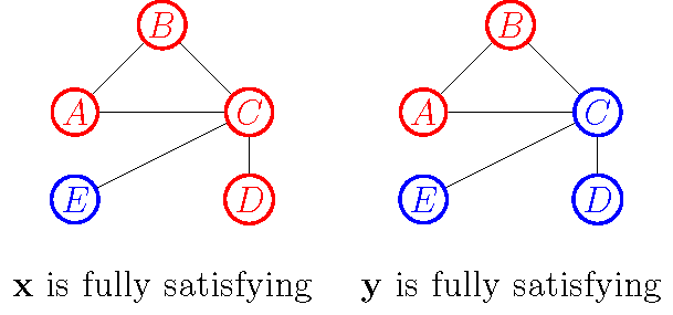
The left panel of
(Orlova’s analysis assumes a fixed underlying network; an interesting follow-up work that need not depart from the fixed-network case could provide a model of preference change, given a fixed network. Such work could be very fruitful for understanding preference conformation or ‘sour-grapes’ type of preference formation à la Jon Elster. For example, assume that agents care about (at least feeling like they are) staying true to their preference—agents exhibit, we might say, a genuineness bias. Then, a frustrating equilibrium imposes a (psychological) penalty that a satisfying one doesn’t. If agents adjust their preferences in a way that makes the optimality of being genuine more likely, then a dynamic model of preference change could explain how, and under what conditions, agents may move from an unstable to a stable fully satisfying equilibrium (say, from the left panel to the right panel of
What about heterogenous frustrating equilibria? Consider a heterogenous profile, where at least two agents are taking different actions. Suppose that the two actions are (drinking) coffee and (drinking) tea. We may split, or partition, the set of agents into two disjoint sets: (1) those who choose coffee (\(S^{c}\)), and (2) those who choose tea (\(S^{t}\)). We may further split each of these sets into two subsets: those who are satisfied, given their action, and those who are frustrated. Thus, the set of coffee-drinkers \(S^{c} = S^{cc} \cup S^{ct}\) can be partitioned into the set of satisfied coffee-drinkers \(S^{cc}\) (who prefer coffee) and the set of frustrated coffee-drinkers \(S^{ct}\) (who prefer tea). Similarly, for the set of tea-drinkers \(S^{t} = S^{tt} \cup S^{tc}\). In part (ii) of Theorem 1 (37), Orlova shows that a heterogenous profile (including a frustrating profile) is an equilibrium if and only if the agents in the satisfied (\(S^{cc}\) and \(S^{tt}\)) and the frustrated (\(S^{ct}\) and \(S^{tc}\)) sets meet certain ‘connectivity’ conditions. More precisely, (1) all satisfied agents of degree \(d_{i}\) need to have at least \(l_{\delta,\lambda}(d_{i})\) neighbours who perform the same action (drink the same beverage), and (2) all frustrated agents of degree \(d_{i}\) need to have at least \(d_{i} - l_{\delta,\lambda}(d_{i}) + 1\) neighbours who perform the same action (drink the same beverage). Combining this with the observation about \(l_{\delta,\lambda}(d_{i})\) above, we may say that, ceteris paribus, the higher one’s degree is (the more ‘popular’ one is), the easier it is to be optimally satisfied and the harder it is to be optimally frustrated—it is easier (harder) for more ‘popular’ agents to optimally follow (go against) their preferences.
One implication of these conditions is that, given the ‘clique-ish’ preferences in the right panel of
There is thus an interesting interplay between the structure of the network and the underlying preference distribution that together determine whether a frustrating profile, where at least some agent(s) go against their preference, is an equilibrium. (In Figure 8b, 43, Orlova gives an example where a heterogeneous frustrating equilibrium does exist.) On the other hand, as Orlova points out (38), the existence of fully satisfying equilibria, while crucially dependent on the distribution of preferences, may also crucially depend on the structure of a network (Orlova’s example here is star networks where, when preferences are heterogenous, a fully satisfying equilibrium never exists; see also the discussion of efficiency in such networks on 40).
Anti-coordination games
The case of anti-coordination games, where \(0 \leq \delta < 1/2\) and \(0 < \lambda < 1 - 2\delta\), is inversely analogous to that of coordination games. We may thus summarise the results in this case more quickly.
First, in anti-coordination games, we no longer speak of companions but of opponents—neighbours who perform an agent’s dispreferred action. Thus, \(l_{\delta,\lambda}(d_{i})\) now gives the minimum number of opponents an agent needs for the optimality of her preferred action. In our five-agent network, \(l_{\delta,\lambda}(d_{i})\) for the three degree values is now given by (notice that the upper bound of the idiosyncratic benefit is now \(1 - 2\delta > 0\)):
Degree \(1\):
(1) \(l_{\delta,\lambda}(1) = \lambda + 1 - 2 \delta\) when \((1 - 2\delta)\frac{1-2(1 - 2\delta)}{1+2(1 - 2\delta)} \leq \lambda < 1 - 2\delta\);
(2) \(l_{\delta,\lambda}(1) = \lambda + 2 - 2 \delta\) when \(0 < \lambda < (1 - 2\delta)\frac{1-2(1 - 2\delta)}{1+2(1 - 2\delta)}\).
Degree \(2\):
(1) \(l_{\delta,\lambda}(2) = \lambda\) when \((1 - 2\delta)\frac{1}{2 - 2\delta} \leq \lambda < 1 - 2\delta\);
(2) \(l_{\delta,\lambda}(2) = \lambda + 1\) when \(0 < \lambda < (1 - 2\delta)\frac{1}{2 - 2\delta}\).
Degree \(3\):
(1) \(l_{\delta,\lambda}(4) = \lambda - \frac{1 - 2\delta}{2}\) when \((1 - 2\delta)\frac{1 + \frac{1 - 2\delta}{4}}{1 + \frac{1 - 2\delta}{2}} \leq \lambda < 1 - 2\delta\);
(1) \(l_{\delta,\lambda}(4) = \lambda - \frac{1 - 2\delta}{2} + 1\) when \(0 < \lambda < (1 - 2\delta)\frac{1 + \frac{1 - 2\delta}{4}}{1 + \frac{1 - 2\delta}{2}}\).
And, again, notice that, ceteris paribus, the more ‘popular’ an agent is—in the sense of having more friends—the fewer opponents she needs for her preferred action to be optimal, that is, for more connected agents, it is easier to optimally follow their preferences.
Theorem 3 (38) establishes the conditions for the existence of equilibria in anti-coordination games: (1) homogeneous equilibria never exist (as in the non-idiosyncratic case), and (2) a heterogenous equilibrium exists if and only if (2.1) satisfied agents of degree \(d_{i}\) (above, in the sets \(S^{cc}\) and \(S^{tt}\)) have at least \(l_{\delta,\lambda}(d_{i})\) neighbours who perform a different action, and (2.2) frustrated agents of degree \(d_{i}\) (above, in the sets \(S^{ct}\) and \(S^{tc}\)) have at least \(d_{i} - l_{\delta,\lambda}(d_{i}) + 1\) neighbours who perform a different action.
Since in anti-coordination games, players have anti-coordination incentives, the existence of a fully satisfying equilibrium—still crucially dependent on the preference distribution—depends on there being sufficient ‘clique-ish’ heterogeneity in the agents’ preferences. More precisely, a fully satisfying equilibrium exists if and only if each agent of degree \(d_{i}\) has at least \(l_{\delta,\lambda}(d_{i})\) neighbours with a different preference.
(Orlova provides two other characterisations of the existence conditions for equilibria in coordination (37–38) and anti-coordination (39) games. These are glossed over here.)
Identity choice
One, among many, interesting interpretations of Orlova’s framework is that of identity choice. Particularly, the model can be interpreted as a model of both personal and social identity. In the case of personal identity, the nodes (players) in the network can be taken to be distinct normative principles that are important to an agent. Connections between nodes can be taken to be some pre-existing (say, coherence) connections between the principles. Each principle then yields a binary ranking of two alternatives—the node’s ‘preference’ over the two alternatives—which may be interpreted as standing for the approval and disapproval of a certain, say, action (such as killing, lying, and so on; of course, the relevant objects need not be actions—they could be, for example, character features that are deemed, according to the relevant principle, to be virtues or vices). ‘Preferences’ here then stand for the verdicts given by the principles in question, which are related to each other according to the network. (‘Popular’ principles ‘cohere’ with a higher number of other principles.) Under heterogenous preferences, we have intrapersonal (normative) conflict where principles that the agent finds important pull in different directions. What about the interpretation of ‘actions’? These may vary but an interesting one is the following. Suppose that ‘normative’ means ‘rational’. Given diverging verdicts about what the rational thing to do is, the agent must come to an all-things-considered verdict: namely, that the action in question is the rational thing to do or not. Under this interpretation, the ‘ideal’ cases, which an agent can find herself in, are those of homogeneous equilibria. Here, these would be cases where the agent does reach an all-things-considered verdict (it would be frustrating for some principles if there were normative conflict). Heterogenous equilibria, on the other hand, would be cases where the agent cannot reach an all-things-considered verdict—in fully satisfying heterogenous equilibria, the agent agrees with the verdict of each principle but these verdicts disagree; in the case of frustrating heterogenous equilibria, not only does the agent fail to reach an all-things-considered verdict, but she also fails to agree (perhaps for good reason) with the principles in question. Heterogenous equilibria thus pose distinct problems depending on whether they are satisfying or frustrating.
Here, I’ll take up the more natural interpretation of Orlova’s model as one of social identity choice. Under this interpretation, the agents are individuals and the connections between them are, say, friendship relations. Each individual may join either of two groups and each individual prefers one of the two groups to the other. (This model is then an extension of Dasgupta and Goyal’s model of narrow identities to a network framework.) Under this interpretation, homogeneous (heterogenous) profiles are profiles where everyone (at least someone) joins the same (a different) group. Fully satisfying profiles are profiles where everyone joins their preferred group and so can be said to ‘stay true’ to their preferences; while frustrating profiles are profiles where at least some agents go against their preferences. Interactional effects thus refer to ‘social pressure’ effects and these may or may not be offset by sufficiently high idiosyncratic effects.